Binomial proportion confidence interval

In statistics, a binomial proportion confidence interval is a confidence interval for a proportion in a statistical population. It uses the proportion estimated in a statistical sample and allows for sampling error. There are several formulas for a binomial confidence interval, but all of them rely on the assumption of a binomial distribution. In general, a binomial distribution applies when an experiment is repeated a fixed number of times, each trial of the experiment has two possible outcomes (labeled arbitrarily success and failure), the probability of success is the same for each trial, and the trials are statistically independent.

A simple example of a binomial distribution is the set of various possible outcomes, and their probabilities, for the number of heads observed when a (not necessarily fair) coin is flipped ten times. The observed binomial proportion is the fraction of the flips which turn out to be heads. Given this observed proportion, the confidence interval for the true proportion innate in that coin is a range of possible proportions which may contain the true proportion. A 95% confidence interval for the proportion, for instance, will contain the true proportion 95% of the times that the procedure for constructing the confidence interval is employed.

There are several ways to compute a confidence interval for a binomial proportion. The normal approximation interval is the simplest formula, and the one introduced in most basic Statistics classes and textbooks. This formula, however, is based on an approximation that does not always work well. Several competing formulas are available that perform better, especially for situations with a small sample size and a proportion very close to zero or one. The choice of interval will depend on how important it is to use a simple and easy-to-explain interval versus the desire for better accuracy.

1 Normal approximation interval
2 Wilson score interval
3 Clopper-Pearson interval
4 Agresti-Coull Interval
5 Jeffreys interval
6 Comparison of different intervals
7 See also
8 References
9 Further reading

Normal approximation interval

The simplest and most commonly used formula for a binomial confidence interval relies on approximating the binomial distribution with a normal distribution. This approximation is justified by the central limit theorem. The formula is

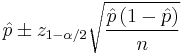
$\hat p \pm z_{1- \alpha /2} \sqrt{ \frac{\hat p \left ( 1- \hat p \right )}{n}}$

where $\hat p$ is the proportion of successes in a Bernoulli trial process estimated from the statistical sample, $z_{1- \alpha /2}$ is the $1- \alpha /2$ percentile of a standard normal distribution, $\alpha$ is the error percentile and n is the sample size. For example, for a 95% confidence level the error ( $\alpha$ ) is 5%, so $1- \alpha /2=0.975$ and $z_{1- \alpha /2}=1.96$ .

The central limit theorem applies well to a binomial distribution, even with a sample size less than 30, as long as the proportion is not too close to 0 or 1. For very extreme probabilities, though, a sample size of 30 or more may still be inadequate. The normal approximation fails totally when the sample proportion is exactly zero or exactly one. A frequently cited rule of thumb is that the normal approximation works well as long as np > 5 and n(1 − p) > 5; see however Brown et al. 2001.^[1] In practice there is little reason to use this method rather than one of the other, better performing, methods.

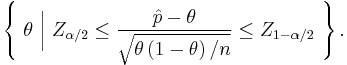
An important theoretical derivation of this confidence interval involves the inversion of a hypothesis test. Under this formulation, the confidence interval represents those values of the population parameter that would have large p-values if they were tested as a hypothesized population proportion. The collection of values, $\theta$ , for which the normal approximation is valid can be represented as

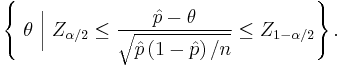
$\left \{\ \theta \ \bigg| \ Z_{\alpha / 2} \le \frac{{\hat p - \theta}}{{\sqrt{\hat p \left ( {1-\hat p} \right ) / n}}} \le Z_{1-\alpha / 2} \right \}.$

Since the test in the middle of the inequality is a Wald test, the normal approximation interval is sometimes called the Wald interval, but Pierre-Simon Laplace described it 1812 in Théorie analytique des probabilités (pag. 283).

Wilson score interval

The Wilson interval is an improvement (the actual coverage probability is closer to the nominal value) over the normal approximation interval and was first developed by Edwin Bidwell Wilson (1927).^[2]

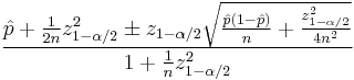
$\frac{{ {\hat p %2B \frac{{1}}{{2n}} z_{1- \alpha / 2}^2 \pm z_{1- \alpha / 2} \sqrt {\frac{{\hat p\left( {1 - \hat p} \right)}}{n} %2B \frac{{z_{1- \alpha / 2}^2}} {{4n^2}} }} }} {{ {1 %2B \frac{{1}}{n}} z_{1- \alpha / 2}^2 }}$

This interval has good properties even for a small number of trials and/or an extreme probability. The center of the Wilson interval

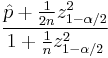
$\frac{{ {\hat p %2B \frac{{1}}{{2n}} z_{1- \alpha / 2}^2 } }} {{ {1 %2B \frac{{1}}{n}} z_{1- \alpha / 2}^2 }}$

can be shown to be a weighted average of $\hat p = X/n$ and $1/2$ , with $\hat p$ receiving greater weight as the sample size increases. For the 95% interval, the Wilson interval is nearly identical to the normal approximation interval using 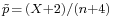$\scriptstyle \tilde p\, =\,(X%2B2)/(n%2B4)$ instead of $\hat p$ .

The Wilson interval can be derived from

$\left \{ \ \theta \ \bigg| \ Z_{\alpha / 2} \le \frac{{\hat p - \theta}}{{\sqrt{\theta \left ( {1-\theta} \right ) / n}}} \le Z_{1-\alpha / 2}\ \right \}.$

by solving for $\theta$ .

The test in the middle of the inequality is a score test, so the Wilson interval is sometimes called the Wilson score interval.

Clopper-Pearson interval

The Clopper-Pearson interval is an early and very common method for calculating binomial confidence intervals.^[3] This is often called an 'exact' method, but that is because it is based on the cumulative probabilities of the binomial distribution (i.e. exactly the correct distribution rather than an approximation), but the intervals are not exact in the way that one might assume: the discontinuous nature of the binomial distribution precludes any interval with exact coverage for all population proportions. The Clopper-Pearson interval can be written as

$\left \{\ \theta \ \Big| \ P \left [ \mathrm{Bin} \left ( n; \theta \right ) \le X \right ] \ge \alpha /2 \right \}\ \bigcap\ \left \{\ \theta\ \Big|\ P \left [ \mathrm{Bin} \left ( n; \theta \right ) \ge X \right ] \ge \alpha /2 \ \right \}$

where X is the number of successes observed in the sample and Bin(n; θ) is a binomial random variable with n trials and probability of success θ.

Because of a relationship between the cumulative binomial distribution and the beta distribution, the Clopper-Pearson interval is sometimes presented in an alternate format that uses percentiles from the beta distribution. The beta distribution is, in turn, related to the F-distribution so a third formulation of the Clopper-Pearson interval uses F percentiles.

The Clopper-Pearson interval is an exact interval since it is based directly on the binomial distribution rather than any approximation to the binomial distribution. This interval never has less than the nominal coverage for any population proportion, but that means that it is usually conservative. For example, the true coverage rate of a 95% Clopper-Pearson interval may be well above 95%, depending on n and θ. Thus the interval may be wider than it needs to be to achieve 95% confidence. In contrast, it is worth noting that other confidence bounds may be narrower than their nominal confidence with, i.e., the Normal Approximation (or "Standard") Interval, Wilson Interval,^[2] Agresti-Coull Interval,^[4] etc., with a nominal coverage of 95% may in fact cover less than 95%.^[1]

Agresti-Coull Interval

The Agresti-Coull interval is another approximate binomial confidence interval.^[4]

Given $X$ successes in $n$ trials, define

$\tilde{n} = n %2B z_{1- \alpha /2}^2$

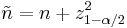
and

$\tilde{p} = \frac{X %2B z_{1- \alpha /2}^2/2}{\tilde{n}}$

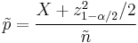
Then, a confidence interval for $p$ is given by

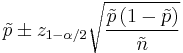
$\tilde{p} \pm z_{1- \alpha /2} \sqrt{\frac{\tilde{p}\left(1 - \tilde{p} \right)}{\tilde{n}}}$

where $z_{1- \alpha /2}$ is the $1- \alpha /2$ percentile of a standard normal distribution, as before. For example, for a 95% confidence interval, let $\alpha = 0.05$ , so $z_{1- \alpha /2}$ = 1.96 and $z_{1- \alpha /2}^2$ = 3.84. If we use 2 instead of 1.96 for $z_{1- \alpha /2}$ , this is the "add 2 successes and 2 failures" interval in ^[4]

Jeffreys interval

The 'Jeffreys interval' is the Bayesian credible interval obtained when using the non-informative Jeffreys prior for the binomial proportion $p$ . The Jeffreys prior for this problem is a Beta distribution with parameters $(1/2, 1/2)$ . After observing $x$ successes in $n$ trials, the posterior distribution for $p$ is a Beta distribution with parameters $(x + 1/2, n - x + 1/2)$ . When $x \neq0$ and $x \neq n$ , the Jeffreys interval is taken to be the $100(1 - α)%$ equal-tailed posterior probability interval, i.e. the $α / 2$ and $1 - α / 2$ quantiles of a Beta distribution with parameters $(x + 1/2, n - x + 1/2)$ . These quantiles need to be computed numerically. In order to avoid the coverage probability tending to zero when $p \to 0$ or $1$ , when $x = 0$ the upper limit is calculated as before but the lower limit is set to 0, and when $x = n$ the lower limit is calculated as before but the upper limit is set to 1.^[1]

Comparison of different intervals

There are several research papers that compare these and other confidence intervals for the binomial proportion. A good starting point is Agresti and Coull (1998)^[4] or Ross (2003)^[5] which point out that exact methods such as the Clopper-Pearson interval may not work as well as certain approximations. But it is still used today for many studies.

References

^ ^a ^b ^c Brown, Lawrence D.; Cai, T. Tony; DasGupta, Anirban (2001). "Interval Estimation for a Binomial Proportion". Statistical Science 16 (2): 101–133. doi:10.1214/ss/1009213286. MR 1861069. Zbl 02068924.
^ ^a ^b Wilson, E. B. (1927). "Probable inference, the law of succession, and statistical inference". Journal of the American Statistical Association 22: 209–212. JSTOR 2276774.
^ Clopper, C.; Pearson, E. S. (1934). "The use of confidence or fiducial limits illustrated in the case of the binomial". Biometrika 26: 404–413. doi:10.1093/biomet/26.4.404.
^ ^a ^b ^c ^d Agresti, Alan; Coull, Brent A. (1998). "Approximate is better than 'exact' for interval estimation of binomial proportions". The American Statistician 52: 119–126. doi:10.2307/2685469. JSTOR 2685469. MR 1628435.
^ Ross, T. D. (2003). "Accurate confidence intervals for binomial proportion and Poisson rate estimation". Computers in Biology and Medicine 33: 509–531. doi:10.1016/S0010-4825(03)00019-2.